A big part of the later stages of beta prototyping for us has been designing and implementing testing procedures for a variety of performance metrics, including airflow, temperature, and damper control. The beta prototype was tested and analyzed in a variety of ways. We performed physical testing as well as CAD and CFD analysis on the system.
The entire system, consisting of both the thermal storage component and thermal comfort component, was tested over an approximately 8 hour period. Before being tested, the entire experimental setup underwent some preparatory actions including:
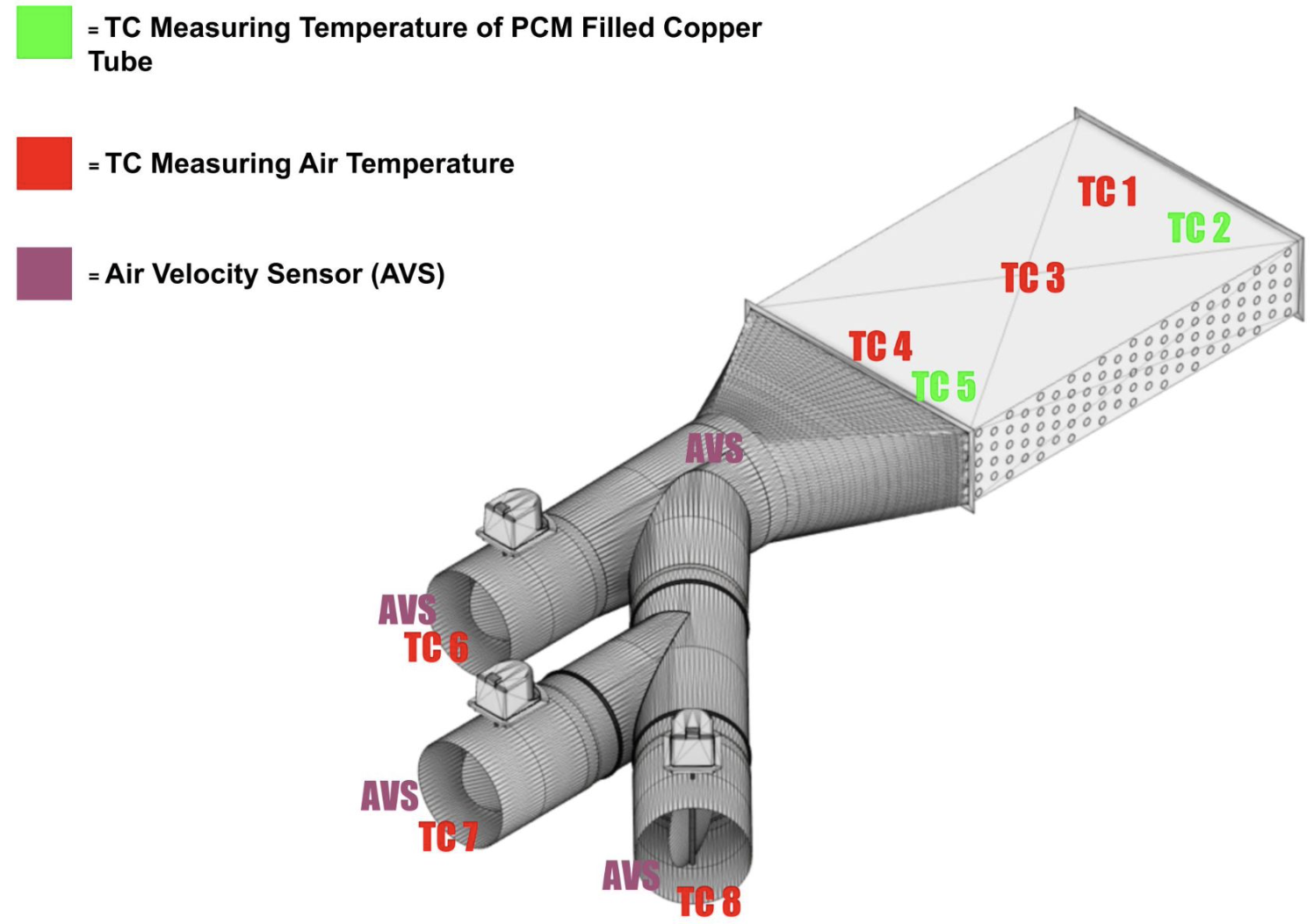
- Installing thermocouples and air velocity sensors (see figure for relative locations).
- Covering the sides of the heat exchanger with an airtight garbage bag to prevent air leakage.
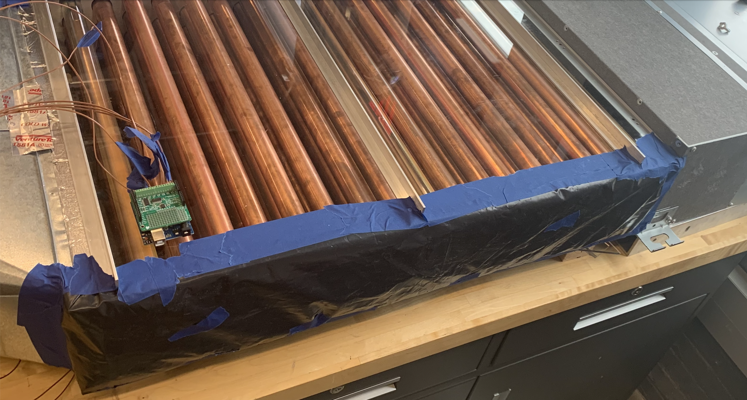
- Using aluminum tape to make the transitions from piece-to-piece more smooth and to prevent air leakage.
- Opening the dampers to maximum airflow position (kept fully open during testing).
- Measuring the ambient air temperature (73 F).
The testing procedure consisted of starting the HVAC system by turning on the compressor (to supply cool air), setting the fan speed of the HVAC system to maximum, and turning on the booster fan. After approximately 3 hours, the compressor was turned off and the fans were left on. After another approximately 5 hours, the entire HVAC system was turned off and data was collected. Airspeeds out of the three ducts ranged from 0.1 m/s to 1.4 m/s. The thermocouple data was filtered and analyzed in MATLAB. The 3 most interesting thermocouples to analyze was the thermocouple at the inlet of the heat exchanger in the air, the thermocouple at the outlet of the heat exchanger in the air, and the thermocouple at the outlet of the heat exchanger on the tube. Below is a picture of the data for these 3 thermocouples:
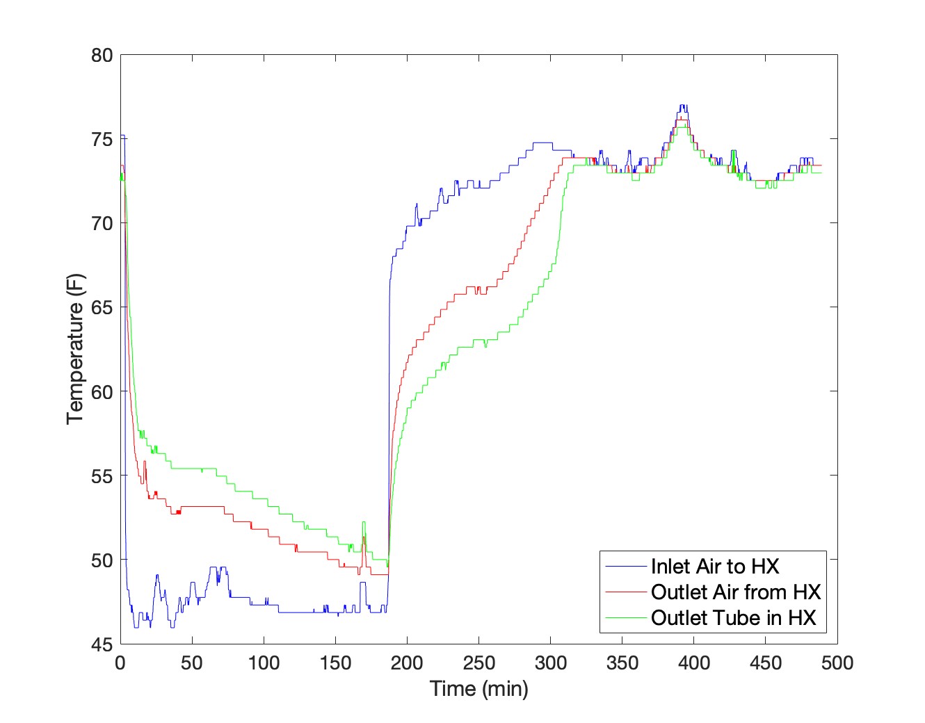
The graph shows that the temperature of the inlet air spiked around 180 minutes which is when the compressor was turned off. However, the performance of our PCM is shown by the fact that for 128 minutes after the compressor was turned off, the temperature of the air being output from the heat exchanger was cooler than the ambient air temperature. This means our system has 128 minutes of cooling capability when charged for around 180 minutes. Calculations of energy required to charge the heat exchanger amount of energy discharged from the heat exchanger showed that the system’s round trip efficiency was 85.3%. It’s important to note that this was done without insulation and without any pause between the charging phase and discharging phase which would be common in household use.
Using electricity rates in Santa Barbara, which charges 0.24 $/kWh during off-peak hours and 0.62 $/kWh during on-peak hours, our system can save up to $23.36 per day. This is because our system can allow for the compressor to be turned off for around 128 minutes per day, resulting in a savings of 28.76 kWh per day.
An interesting observation from the graph is that around 56 F from about 50 minutes to 75 minutes, the temperature of the outlet air and outlet tube remain almost constant. This could be explained by the fact that the PCM was transitioning from liquid to solid. The manufacturer’s published freezing point for the PCM is 59 F, so it’s reasonable to assume that we are seeing a phase change at 56 F on the graph. In future testing, the team would like to test the heat exchanger again but only charge it for around 75 minutes because any additional charging will go to sensible heat transfer rather than latent heat transfer. This may result in better round trip efficiency and will require less energy during charging.
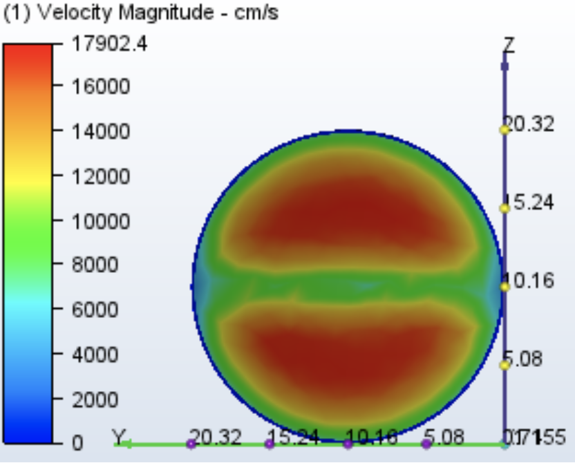
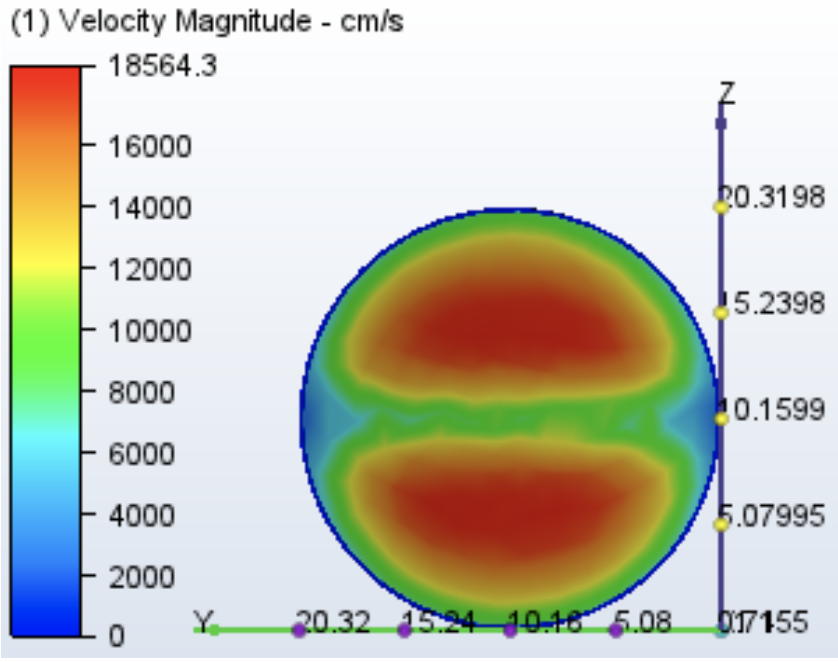
Moving on to the airflow analysis, we decided to calculate the air velocity at four points in our system (seen in the previous picture above). The first point was after the booster fan but before the ductwork split. The other three points were located after each damper. In order to collect data, we first ordered a pitot tube made specifically for HVAC circular ducts. Then, using tubing, we connected the pitot tube to a differential pressure sensor and used an arduino to get differential pressure values. Finally, Bernoulli’s equation was used to calculate the air velocity.
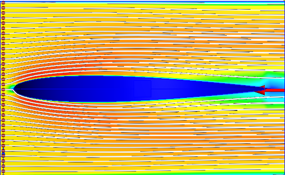
As for the airfoil damper, the following results were found:
Conventional Damper
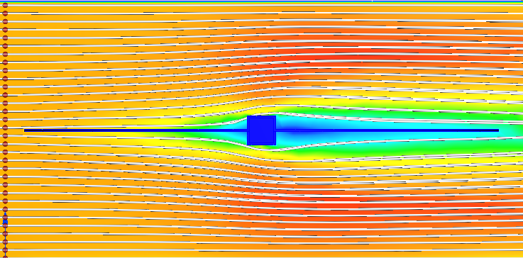
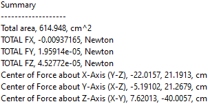
Coefficient of Drag: 0.12
Helios Damper
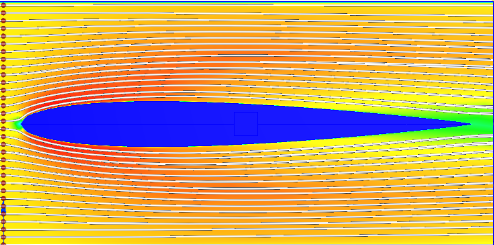
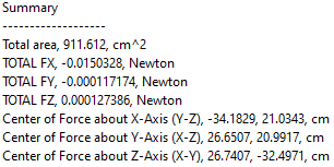
Coefficient of Drag: 0.13
These two simulations were run with both damper models at the same circular top down dimensions. The diameter for both models were 7.2 in^2. As calculated from the simulation, the drag coefficient is higher for the helios damper in comparison to the conventional damper. After analyzing these results, the damper was scaled down to 0.8 the original size and the following results were achieved.
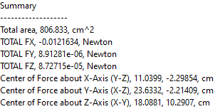
Coefficient of Drag: 0.11
For the next steps in our airfoil design, we first need to calculate the amount of allotted pressure when the damper is in its fully closed position. After this, the necessary cross sectional area of the damper can be calculated.
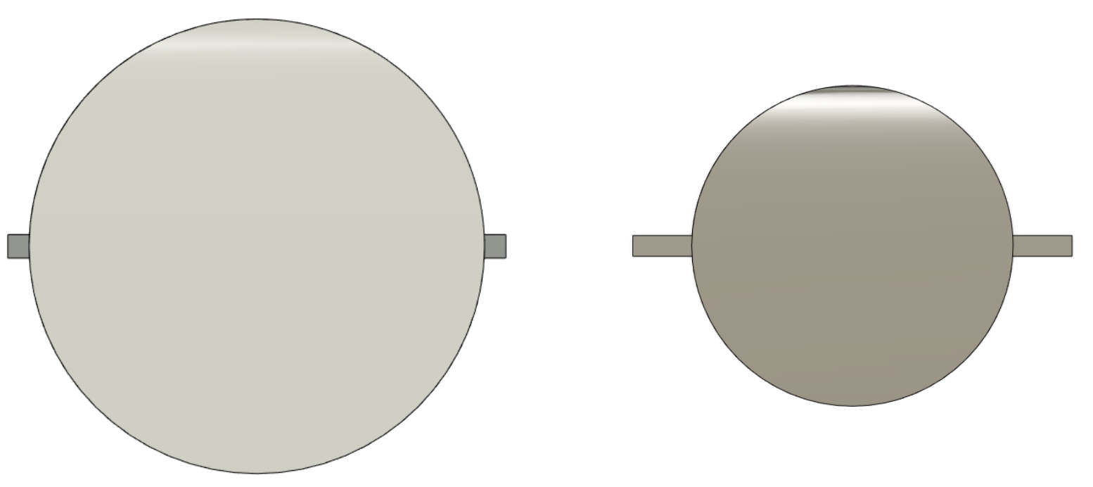
In addition, here is a comparison of the current versus scaled down versions of the airfoil damper. The rectangular axel is the same for scale. The scaled down version has an improved coefficient of drag versus the conventional but at the cost of 20% of the topdown surface area. In order to gain some of this surface area back without impacting the drag coefficient, the scaled down version must be widened without increasing the height.
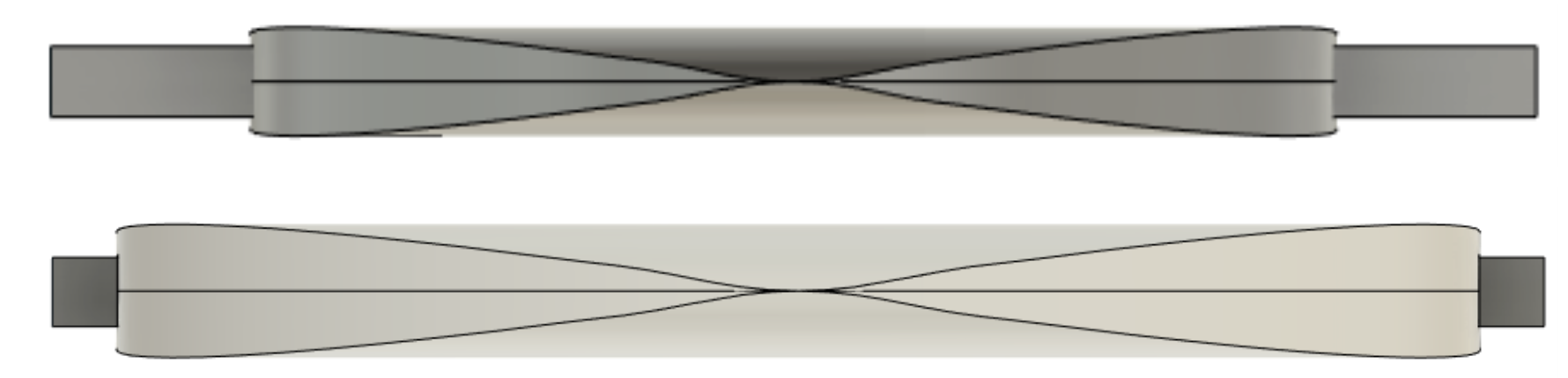
The final version of the airfoil damper would instead need to look like this in order to have a lower drag coefficient than the conventional damper at 0 degrees:
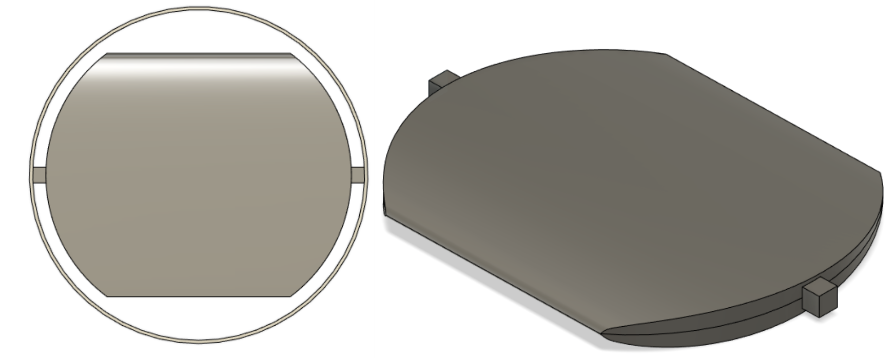
Overall, this shows that the NA0100 airfoil shape can reduce pressure drop for our system, but at the cost of surface area to block airflow when in the fully closed position.